
 By Ashwini Joshi
For small sample data or rare events data, exact non-parametric tests perform better than asymptotic tests. But they come with the disadvantage of conservativeness. Many corrections have been suggested to reduce this conservativeness but none of them solve the problems entirely. StatXact provides various methods of computing exact p-values. Depending upon the problem at hand, the user can decide which one to use.
Let’s consider a hypothetical example of stratified count data. The example shows two sample data with two strata. Events in Treatment1 are rare as compared to the ones in Treatment0. But the event rates are comparable.
|
Treatment |
Stratum |
Events |
Follow-up time |
Event Rate |
|
Treatment0 |
1 |
10 |
3075.27 |
0.003251747 |
|
Treatment1 |
1 |
0 |
337.29 |
0 |
|
Treatment0 |
2 |
10 |
3075.27 |
0.003251747 |
|
Treatment1 |
2 |
1 |
337.29 |
0.002964808 |
For such data of rare events, asymptotic results may not be reliable. But finding the Exact non-parametric distribution is not an easy task.
Let’s see how to compute exact non-parametric distribution…
Exact non-parametric distribution is a discrete distribution. Keeping total events in each stratum fixed, enumerate all possible combinations of events in treatment 0 and treatment1. If Treatment1 is a treatment of interest then consider the number of events in Treatment1 as a test statistic for each stratum. One can decide any other value as test statistic which will uniquely represent the combination in the above said enumeration. Once we have distribution of test statistic for each stratum we will convolute to get the overall distribution. For each test statistic compute the point probability. The point probability is the probability of getting exactly the observed test statistic, i.e. p (Test statistic= ‘Observed Test statistic’). In our example we need to go through all possible counts of Treatment0 and Treatment1, in stratum 1 that sums up to 10 and compute the ratio of rates for each of these pairs of values; do the same for all possible counts of Treatment0,Treatment1, in stratum 2 that sums up to 11.
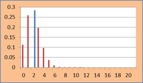
Exact Distribution for this example is shown below:
Here Test Statistic is total number of events observed in Treatment1.
Exact Distribution:
|
Statistic |
Point Probability |
|
0 |
0.112425 |
|
1 |
0.258941 |
|
2 |
0.284002 |
|
3 |
0.197276 |
|
4 |
0.097366 |
|
5 |
0.036308 |
|
6 |
0.010619 |
|
7 |
0.002496 |
|
8 |
4.79E-04 |
|
9 |
7.59E-05 |
|
10 |
9.99E-06 |
|
11 |
1.10E-06 |
|
12 |
1.00E-07 |
|
13 |
7.60E-09 |
|
14 |
4.76E-10 |
|
15 |
2.44E-11 |
|
16 |
1.00E-12 |
|
17 |
3.24E-14 |
|
18 |
7.89E-16 |
|
19 |
1.37E-17 |
|
20 |
1.50E-19 |
|
21 |
7.82E-22 |
The next task is to compute p-value from this distribution.
Depending upon the definition of rejection region, p-value computation differs. Let ‘t’ represent the observed value of test statistic. In this example t is 1.
1-Sided p-value is computed as: min (p (T>= t), p (T<= t))
In this example, observed value of test statistic is 1. Its 1-sided p-value is p (T<= 1) = 0.371366.
Graphically it can be represented as:
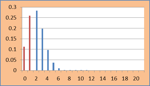
‘RED’ color represents the rejection region from which p-value is computed.
To reduce the conservativeness, Mid-p corrected p-value is used which can be easily obtained by
(1-sided p-value) – (point probability of t)/2
In this example it is 0.241896.
Graphically it can be represented as:
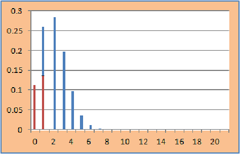
Here half of the point probability of t (Test statistic =1) is in rejection region (RED) and half of it is outside rejection region (BLUE).
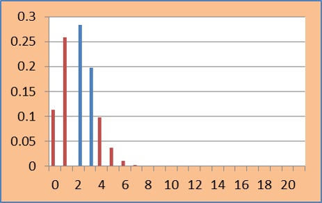
2-sided p-value can be computed in many ways:
- Using 1-sided p-value i.e. 2*(1-sided p-value). In this example it is 0.742732
- Method similar to Asymptotic: Rejection region includes points which are away from mean as compared to observed value. Here mean value of test statistic is 2.076 and observed value is 1. Hence 2 –sided p-value is 0.5187214 as shown below:
- Consider those test statistic values that are less likely observed as compared to t. Rejection region includes points which have point probability less than that of the observed value. Point probability of t is 0.258941 shown by a black horizontal line in the plot. Hence 2-sided p-value is: 0.715998
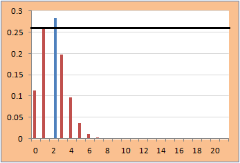
- Blaker’s p-value - Blaker (2000) defines the p-value as the sum of the tail probability in the observed tail plus the largest tail probability in the opposite tail that is not greater than the observed tail probability. In this case it is same as earlier 0.715998.
So it seems straight forward to compute these exact p-values. The problem starts when data is large but sparse. In such cases, enumerating all possible combinations becomes difficult.
At this point specialist software like StatXact comes into its own. StatXact computes the exact distribution implicitly and gives the exact p-value and confidence interval to the user in a reasonable time.
We considered the subset of data from the US national Medicare inpatient hospital database (Medpar) for the 1991 Medicare files for the state of Arizona. The study investigates specific cardiovascular conditions for patients and the data set consists of 1495 observations.
If all the combinations/tables are to be enumerated the number goes beyond 14000.
StatXact created the exact distribution of 14733 distribution points and the hypothesis testing results in only 1.5 seconds on a 64 bit Win 7 machine.
To request a trial of StatXact click the button below.

About the Author
Ashwini Joshi is a subject matter expert in mathematics at Cytel. She received an MSc from IIT Bombay and has been an Assistant Professor in Mathematics at the PVG College of Engineering and Technology.